The AI Crossroad: Hype vs. Practicality
In the modern era of artificial intelligence, Deep Learning (DL) dominates the headlines. From generative AI creating hyper-realistic images to large language models writing code, neural networks seem to be the universal answer to every problem. However, in the trenches of real-world software engineering and data science, throwing a massive neural network at every dataset is a recipe for wasted compute power, exorbitant cloud hosting bills, and uninterpretable results.
Before the deep learning boom of the 2010s, traditional machine learning algorithms ruled the landscape. Among them, the Support Vector Machine (SVM) was—and remains—one of the most mathematically elegant and practically robust algorithms ever devised. For many enterprise applications, predictive models, and classification tasks, an SVM will outperform a deep neural network while using a fraction of the hardware. This article breaks down the architecture of both approaches, exploring when to leverage the sheer power of Deep Learning and when to rely on the surgical precision of an SVM.
The Anatomy of a Support Vector Machine (SVM)
To understand why SVMs are so powerful, we have to strip away the magic and look at the geometry. At its core, an SVM is a supervised learning algorithm used primarily for classification (though it can be adapted for regression).
Imagine a two-dimensional graph with red dots clustered on one side and blue dots on the other. The goal of an SVM is to draw a line—a “decision boundary”—that separates the red dots from the blue dots. But an SVM doesn’t just draw any line; it calculates the optimal line. It seeks the line that has the maximum margin, meaning the greatest possible distance between the line itself and the nearest data points of both classes.
These nearest data points are called the Support Vectors. They are the critical elements of the dataset; if you removed all other data points except the support vectors, the position of the decision boundary would not change.
Mathematically, if we expand this to multidimensional data, this line becomes a hyperplane. The equation of the hyperplane is defined as:
w^T x + b = 0
where w is the weight vector, x is the input vector, and b is the bias. The algorithm optimizes the model by minimizing ||w||, which effectively maximizes the margin between the two classes.
Conquering Complexity: The Kernel Trick
The classic SVM works flawlessly for linearly separable data (data that can be sliced with a straight line or flat plane). But real-world data is messy and rarely linear. How does an SVM separate a cluster of red dots completely surrounded by a ring of blue dots?
This is where the SVM utilizes its secret weapon: The Kernel Trick.
Instead of trying to draw a complex, squiggly line in the current dimension, a mathematical function (the Kernel) projects the data into a higher-dimensional space. By mapping 2D data into 3D space, that ring of blue dots might suddenly sit “below” the red dots, allowing the SVM to easily slice a flat, 2D plane right between them. Once the calculation is done, it projects the boundary back into the original space.
Common kernels include:
- Linear Kernel: For simple, easily separable data.
- Polynomial Kernel: Projects data into curved dimensional spaces.
- Radial Basis Function (RBF): The most popular non-linear kernel, capable of handling highly complex, overlapping datasets by mapping them into infinite-dimensional space.
The Anatomy of Deep Learning
Deep Learning is a specialized subset of machine learning based on Artificial Neural Networks (ANNs). Inspired by the biological brain, DL models consist of an input layer, an output layer, and multiple “hidden layers” in between—hence the term “deep.”
Unlike an SVM, which uses rigorous geometrical optimization, Deep Learning uses a brute-force mathematical approach called backpropagation. The network is fed raw data, makes a guess, calculates its error (the loss function), and then works backward through the layers to adjust the mathematical weights of thousands or millions of interconnected artificial neurons.
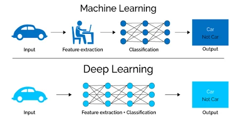
While SVMs excel at drawing boundaries based on existing features, Deep Learning networks are “feature extractors.” They do not require a human data scientist to tell them what variables to look at. If you feed a deep learning model millions of pictures of cars, its initial layers will automatically learn to detect edges; the middle layers will learn to detect wheels and windshields, and the final layers will recognize the entire car.
Head-to-Head: Where SVM Excels
Small to Medium Datasets: This is the SVM’s ultimate playground. Deep Learning models are incredibly data-hungry; training a neural network on a small dataset often leads to “overfitting” (where the model memorizes the training data but fails completely on new data). SVMs, because they rely only on the support vectors, can build highly accurate models with just a few hundred or thousand data points.
Computational Efficiency: You can train an SVM on a standard laptop CPU in seconds or minutes. Training a Deep Learning model often requires expensive, power-hungry GPUs (Graphics Processing Units) or TPUs running for hours, days, or even weeks.
High-Dimensional Data: SVMs are exceptionally good at handling datasets where the number of features (dimensions) exceeds the number of samples. This makes them heavily favored in fields like bioinformatics, such as classifying DNA microarray data.
Interpretability: In regulated industries like finance or healthcare, you must be able to explain why an AI made a specific decision. An SVM’s mathematical boundary can be audited. Deep Learning models are notorious “black boxes”; tracking exactly why a network made a specific choice across billions of parameters is nearly impossible.
Head-to-Head: Where Deep Learning Dominates
Massive, Unstructured Data: When dealing with gigabytes or terabytes of raw images, audio files, or natural language text, SVMs hit a computational wall. Deep Learning scales incredibly well with data; the more data you feed a neural network, the more accurate it becomes.
Zero Manual Feature Engineering: To use an SVM on a dataset of images, a human must first write algorithms to extract features (like color histograms or edge densities) to feed into the SVM. Deep Learning ingests raw pixels and learns the features automatically, saving hundreds of hours of manual engineering.
Complex, Layered Problems: For tasks like real-time translation, generative AI, or complex game environment navigation, the intricate, layered architecture of Deep Learning is the only viable solution. The hierarchical learning of an ANN allows it to capture nuances in data that a geometrical hyperplane simply cannot map.
Making the Choice: A Developer’s Guide
Choosing between an SVM and Deep Learning shouldn’t be based on hype; it should be based on the constraints of your specific project.
- Choose Support Vector Machines if: You have a smaller dataset (under 100,000 rows), you have limited computational resources, your data is highly structured (like database tables or spreadsheets), and you require a model that is stable, reliable, and interpretable.
- Choose Deep Learning if: You have a massive dataset of unstructured data (images, video, text), you have access to GPU hardware, accuracy is the absolute highest priority, and you do not need to explain the internal decision-making process of the algorithm.
Ultimately, the best data scientists and tech professionals don’t strictly favor one over the other. They maintain a diverse toolkit, deploying the elegance of an SVM for surgical precision and unleashing the heavy machinery of Deep Learning only when the problem demands it.